Share
In this blog post
- Setting up PyTorch TorchAudio for Audio Data Augmentation
- Adding Effects for Audio Data Augmentation with PyTorch TorchAudio
- Using Sound Effects in Torchaudio
- Adding Background Noise
- Adding Room Reverberation
- Advanced Resampling of Audio Data with TorchAudio
- Audio Feature Extraction with PyTorch TorchAudio
- In Summary
PyTorch is one of the leading machine learning frameworks in Python. Recently, PyTorch released an updated version of their framework for working with audio data, TorchAudio. TorchAudio supports more than just using audio data for machine learning. It also supports the data transformations, augmentations, and feature extractions needed to use audio data for your machine learning models.
In this post, we'll cover:
Setting up PyTorch TorchAudio for Audio Data Augmentation
At the time of writing, torchaudio is on version 0.11.0 and only works with Python versions 3.6 to 3.9. For this example, we’ll be using Python 3.9. We’ll also need to install some libraries before we dive in. The first libraries we’ll need are torch and torchaudio from PyTorch. We’ll be using matplotlib to plot our visual representations, requests to get the data, and librosa to do some more visual manipulations for spectrograms.
To get started we’ll pip install all of these into a new virtual environment. To start a virtual environment run python3 -m venv <new environment name>. Then run pip install torch torchaudio matplotlib requests librosa and let pip install all the libraries necessary for this tutorial.
Adding Effects for Audio Data Augmentation with PyTorch TorchAudio
Recently, we covered the basics of how to manipulate audio data in Python. In this section we’re going to cover the basics of how to pass sound effect options to TorchAudio. Then, we’ll go into specifics about how to add background noise at different sound levels and how to add room reverb.
Before we get into that, we have to set some stuff up. This section of code is entirely auxiliary code that you can skip. It would be good to understand this code if you’d like to continue testing on the provided data.
In the code block below, we first import all the libraries we need. Then, we define the URLs where the audio data is stored and the local paths we’ll store the audio at. Next, we fetch the data and define some helper functions.
For this example, we’ll define functions to get a noise, speech, and reverb sample. We will also define functions to plot the waveform, spectrogram, and numpy representations of the sounds that we are working with.
import math
import os

import matplotlib.pyplot as plt
import requests
import torchaudio
import torch

_SAMPLE_DIR = "_assets"
SAMPLE_WAV_URL = "https://pytorch-tutorial-assets.s3.amazonaws.com/steam-train-whistle-daniel_simon.wav"
SAMPLE_WAV_PATH = os.path.join(_SAMPLE_DIR, "steam.wav")

SAMPLE_RIR_URL = "https://pytorch-tutorial-assets.s3.amazonaws.com/VOiCES_devkit/distant-16k/room-response/rm1/impulse/Lab41-SRI-VOiCES-rm1-impulse-mc01-stu-clo.wav"  # noqa: E501
SAMPLE_RIR_PATH = os.path.join(_SAMPLE_DIR, "rir.wav")

SAMPLE_WAV_SPEECH_URL = "https://pytorch-tutorial-assets.s3.amazonaws.com/VOiCES_devkit/source-16k/train/sp0307/Lab41-SRI-VOiCES-src-sp0307-ch127535-sg0042.wav"  # noqa: E501
SAMPLE_WAV_SPEECH_PATH = os.path.join(_SAMPLE_DIR, "speech.wav")

SAMPLE_NOISE_URL = "https://pytorch-tutorial-assets.s3.amazonaws.com/VOiCES_devkit/distant-16k/distractors/rm1/babb/Lab41-SRI-VOiCES-rm1-babb-mc01-stu-clo.wav"  # noqa: E501
SAMPLE_NOISE_PATH = os.path.join(_SAMPLE_DIR, "bg.wav")

os.makedirs(_SAMPLE_DIR, exist_ok=True)

def _fetch_data():
   uri = [(SAMPLE_WAV_URL, SAMPLE_WAV_PATH),
           (SAMPLE_RIR_URL, SAMPLE_RIR_PATH),
           (SAMPLE_WAV_SPEECH_URL, SAMPLE_WAV_SPEECH_PATH),
           (SAMPLE_NOISE_URL, SAMPLE_NOISE_PATH),]
   for url, path in uri:
       with open(path, "wb") as file_:
           file_.write(requests.get(url).content)

_fetch_data()

def _get_sample(path, resample=None):
   effects = [["remix","1"]]
   if resample:
       effects.extend([
           ["lowpass", f"{resample // 2}"],
           ["rate", f"{resample}"]
       ])
   return torchaudio.sox_effects.apply_effects_file(path, effects=effects)

def get_sample(*, resample=None):
   return _get_sample(SAMPLE_WAV_PATH, resample=resample)

def get_speech_sample(*, resample=None):
   return _get_sample(SAMPLE_WAV_SPEECH_PATH, resample=resample)

def plot_waveform(waveform, sample_rate, title="Waveform", xlim=None, ylim=None):
   waveform = waveform.numpy()
   num_channels, num_frames = waveform.shape
   time_axis = torch.arange(0, num_frames) / sample_rate

   figure, axes = plt.subplots(num_channels, 1)
   if num_channels == 1:
       axes = [axes]
   for c in range(num_channels):
       axes[c].plot(time_axis, waveform[c], linewidth=1)
       axes[c].grid(True)
       if num_channels > 1:
           axes[c].set_ylabel(f"Channel {c+1}")
       if xlim:
           axes[c].set_xlim(xlim)
       if ylim:
           axes[c].set_ylim(ylim)
   figure.suptitle(title)
   plt.show(block=False)

def print_stats(waveform, sample_rate=None, src=None):
   if src:
       print("-"*10)
       print(f"Source: {src}")
       print("-"*10)
   if sample_rate:
       print(f"Sample Rate: {sample_rate}")
   print("Dtype:", waveform.dtype)
   print(f" - Max:     {waveform.max().item():6.3f}")
   print(f" - Min:     {waveform.min().item():6.3f}")
   print(f" - Mean:    {waveform.mean().item():6.3f}")
   print(f" - Std Dev: {waveform.std().item():6.3f}")
   print()
   print(waveform)
   print()

def plot_specgram(waveform, sample_rate, title="Spectrogram", xlim=None):
   waveform = waveform.numpy()
   num_channels, num_frames = waveform.shape
   figure, axes = plt.subplots(num_channels, 1)
   if num_channels == 1:
       axes = [axes]
   for c in range(num_channels):
       axes[c].specgram(waveform[c], Fs=sample_rate)
       if num_channels > 1:
           axes[c].set_ylabel(f"Channel {c+1}")
       if xlim:
           axes[c].set_xlim(xlim)
   figure.suptitle(title)
   plt.show(block=False)

def get_rir_sample(*, resample=None, processed=False):
   rir_raw, sample_rate = _get_sample(SAMPLE_RIR_PATH, resample=resample)
   if not processed:
       return rir_raw, sample_rate
   rir = rir_raw[:, int(sample_rate*1.01) : int(sample_rate * 1.3)]
   rir = rir / torch.norm(rir, p=2)
   rir = torch.flip(rir, [1])
   return rir, sample_rate

def get_noise_sample(*, resample=None):
   return _get_sample(SAMPLE_NOISE_PATH, resample=resample)
Using Sound Effects in Torchaudio
Now that we’ve set everything up, let’s take a look at how to use PyTorch’s torchaudio library to add sound effects. We’re going to pass a list of list of strings (List[List[Str]]) object to the sox_effects.apply_effects_tensor function from torchaudio.
Each of the internal lists in our list of lists contains a set of strings defining an effect. The first string in the sequence indicates the effect and the next entries indicate the parameters around how to apply that effect. In the example below we show how to add a lowpass filter, augment the speed, and add some reverb. For a full list of sound effect options available, check out the sox documentation. Note: this function returns two return values, the waveform and the new sample rate.
# Load the data
waveform1, sample_rate1 = get_sample(resample=16000)

# Define effects
effects = [
   ["lowpass", "-1", "300"],  # apply single-pole lowpass filter
   ["speed", "0.8"],  # reduce the speed
   # This only changes sample rate, so it is necessary to
   # add `rate` effect with original sample rate after this.
   ["rate", f"{sample_rate1}"],
   ["reverb", "-w"],  # Reverbration gives some dramatic feeling
]
# Apply effects
waveform2, sample_rate2 = torchaudio.sox_effects.apply_effects_tensor(waveform1, sample_rate1, effects)
print_stats(waveform1, sample_rate=sample_rate1, src="Original")
print_stats(waveform2, sample_rate=sample_rate2, src="Effects Applied")
plot_waveform(waveform1, sample_rate1, title="Original", xlim=(-0.1, 3.2))
plot_specgram(waveform1, sample_rate1, title="Original", xlim=(0, 3.04))
plot_waveform(waveform2, sample_rate2, title="Effects Applied", xlim=(-0.1, 3.2))
plot_specgram(waveform2, sample_rate2, title="Effects Applied", xlim=(0, 3.04))
The printout from plotting the waveforms and spectrograms are below. Notice that adding the reverb necessitates a multichannel waveform to produce that effect. You can see the difference in the waveform and spectrogram from the effects. Lowering the speed lengthened the sound. Adding a filter compresses some of the sound (visible in the spectrogram). Finally, the reverb adds noise we can see reflected mainly in the “skinnier” or quieter sections of the waveform.
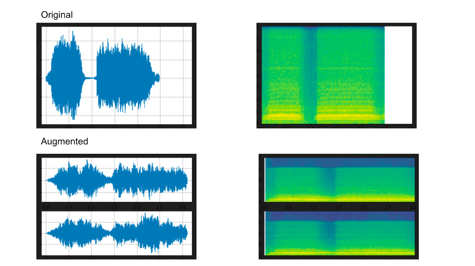 Above: Original Waveform and Spectrogram + Added Effects from TorchAudio
Adding Background Noise
Now that we know how to add effects to audio using torchaudio, let’s dive into some more specific use cases. If your model needs to be able to detect audio even when there’s background noise, it’s a good idea to add some background noise to your training data.
In the example below, we will start by declaring a sample rate (8000 is a pretty typical rate). Next, we’ll call our helper functions to get the speech and background noise and reshape the noise. After that, we’ll use the norm function to normalize both the speech and the text to the second order. Next, we’ll define a list of decibels that we want to play the background noise at over the speech and create a “background noise” version at each level.
sample_rate = 8000
speech, _ = get_speech_sample(resample=sample_rate)
noise, _ = get_noise_sample(resample=sample_rate)
noise = noise[:, : speech.shape[1]]

speech_power = speech.norm(p=2)
noise_power = noise.norm(p=2)

snr_dbs = [20, 10, 3]
noisy_speeches = []
for snr_db in snr_dbs:
   snr = math.exp(snr_db / 10)
   scale = snr * noise_power / speech_power
   noisy_speeches.append((scale * speech + noise) / 2)

plot_waveform(noise, sample_rate, title="Background noise")
plot_specgram(noise, sample_rate, title="Background noise")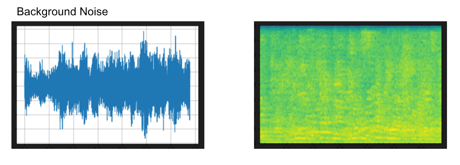
The above pictures show the waveform and the spectrogram of the background noise. We have already created all the noise speech audio data clips in the code above. The code below prints all of them out so we can see what the data looks like at different levels of audio. Note that the 20dB snr means that the signal (speech) to noise (background noise) ratio is at 20 dB, not that the noise is being played at 20 db.
# background noise at certain levels
snr_db20, noisy_speech20 = snr_dbs[0], noisy_speeches[0]
plot_waveform(noisy_speech20, sample_rate, title=f"SNR: {snr_db20} [dB]")
plot_specgram(noisy_speech20, sample_rate, title=f"SNR: {snr_db20} [dB]")
snr_db10, noisy_speech10 = snr_dbs[1], noisy_speeches[1]
plot_waveform(noisy_speech10, sample_rate, title=f"SNR: {snr_db10} [dB]")
plot_specgram(noisy_speech10, sample_rate, title=f"SNR: {snr_db10} [dB]")
snr_db3, noisy_speech3 = snr_dbs[2], noisy_speeches[2]
plot_waveform(noisy_speech3, sample_rate, title=f"SNR: {snr_db3} [dB]")
plot_specgram(noisy_speech3, sample_rate, title=f"SNR: {snr_db3} [dB]")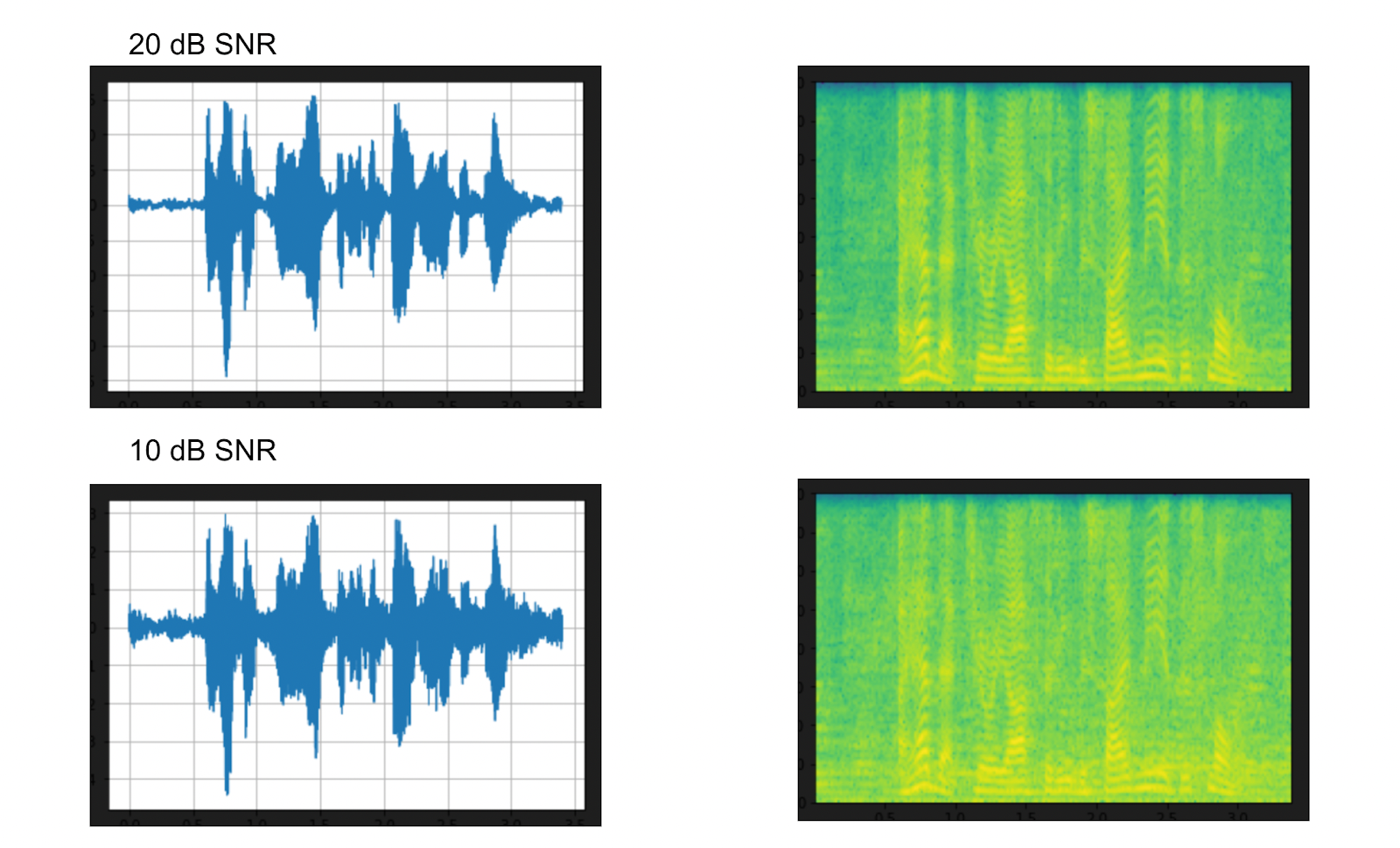 Above: 20 and 10 dB SNR added background noise visualizations via PyTorch TorchAudio
 Above: 3 dB signal to noise ratio waveform and spectrogram for added background noise
Adding Room Reverberation
So far we’ve applied audio effects and background noise at different noise levels. Let’s also take a look at how to add a reverb. Adding reverb to an audio clip gives the impression that the audio has been recorded in an echo-y room. You can do this to make it seem like a presentation you gave to your computer was actually given to an audience in a theater.
To add a room reverb, we’re going to start by making a request for the audio from where it lives online using one of the functions we made above (get_rir_sample). We’ll take a look at the waveform before we clip it to get the “reverb” of the sound, normalize it, and then flip the sound so that the reverb works correctly.
sample_rate = 8000
rir_raw, _ = get_rir_sample(resample=sample_rate)
plot_waveform(rir_raw, sample_rate, title="Room Impulse Response (raw)", ylim=None)
plot_specgram(rir_raw, sample_rate, title="Room Impulse Response (raw)")
rir = rir_raw[:, int(sample_rate * 1.01) : int(sample_rate * 1.3)]
rir = rir / torch.norm(rir, p=2)
rir = torch.flip(rir, [1])
print_stats(rir)
plot_waveform(rir, sample_rate, title="Room Impulse Response", ylim=None)
plot_specgram(rir_raw, sample_rate, title="Room Impulse Response (raw)")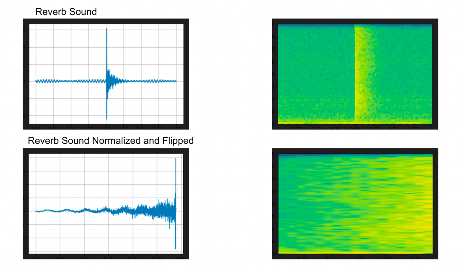 Above: Original and augmented reverb sound visualizations from PyTorch TorchAudio
Once we have the sound normalized and flipped, we’re ready to use it to augment the existing audio. We will first use PyTorch to create a “padding” that uses the speech and the augmented sound. Then, we’ll use PyTorch to apply the sound with a 1 dimensional convolution.
speech, _ = get_speech_sample(resample=sample_rate)
speech_ = torch.nn.functional.pad(speech, (rir.shape[1] - 1, 0))
augmented = torch.nn.functional.conv1d(speech_[None, ...], rir[None, ...])[0]
plot_waveform(speech, sample_rate, title="Original", ylim=None)
plot_specgram(speech, sample_rate, title="Original")
play_audio(speech, sample_rate)
plot_waveform(augmented, sample_rate, title="RIR Applied", ylim=None)
plot_specgram(augmented, sample_rate, title="RIR Applied")
play_audio(augmented, sample_rate)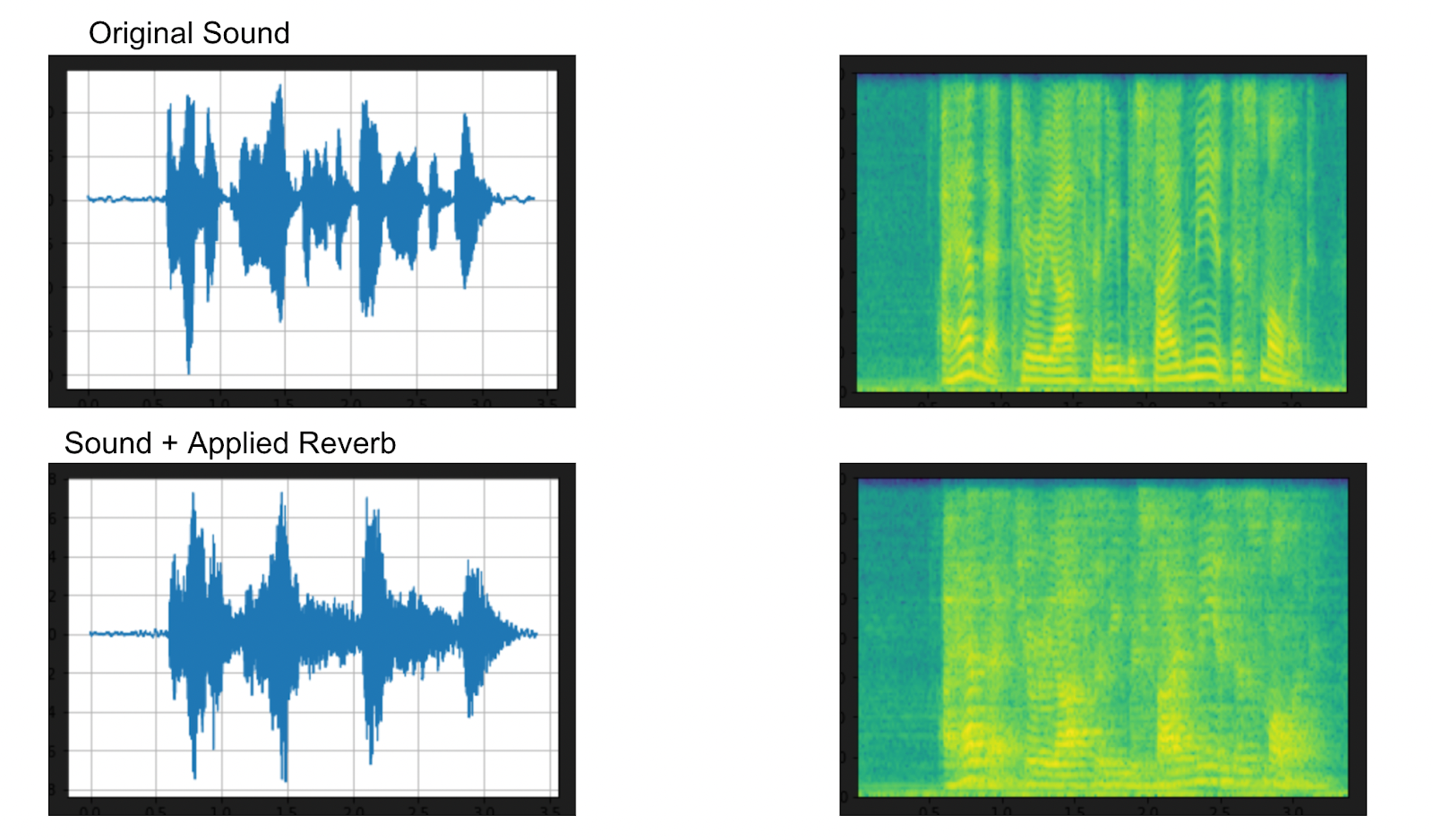 Above: Visualizations for audio with reverb applied by TorchAudio
From the printout above we can see that adding the room reverb adds echo like sounds to the waveform. We can also see that the spectrogram is less defined than it would be for a crisp, next-to-the-mic sound.
Advanced Resampling of Audio Data with TorchAudio
We briefly mentioned how to resample data before using the pydub and the sklearn libraries. TorchAudio also lets you easily resample audio data using multiple methods. In this section, we’ll cover how to resample data using low-pass, rolloff, and window filters.
As we have done above, we need to set up a bunch of helper functions before we get into actually resampling the data. Many of these setup functions serve the same functions as the ones above. The one here to pay attention to is get_sine_sweep which is what we’ll be using instead of an existing audio file. All the other functions like getting ticks and reverse log frequencies are for plotting the data.
import math
import torch

import matplotlib.pyplot as plt
from IPython.display import Audio, display


DEFAULT_OFFSET = 201
SWEEP_MAX_SAMPLE_RATE = 48000
DEFAULT_LOWPASS_FILTER_WIDTH = 6
DEFAULT_ROLLOFF = 0.99
DEFAULT_RESAMPLING_METHOD = "sinc_interpolation"

def _get_log_freq(sample_rate, max_sweep_rate, offset):
   """Get freqs evenly spaced out in log-scale, between [0, max_sweep_rate // 2]

   offset is used to avoid negative infinity `log(offset + x)`.

   """
   start, stop = math.log(offset), math.log(offset + max_sweep_rate // 2)
   return torch.exp(torch.linspace(start, stop, sample_rate, dtype=torch.double)) - offset

def _get_inverse_log_freq(freq, sample_rate, offset):
   """Find the time where the given frequency is given by _get_log_freq"""
   half = sample_rate // 2
   return sample_rate * (math.log(1 + freq / offset) / math.log(1 + half / offset))


def _get_freq_ticks(sample_rate, offset, f_max):
   # Given the original sample rate used for generating the sweep,
   # find the x-axis value where the log-scale major frequency values fall in
   time, freq = [], []
   for exp in range(2, 5):
       for v in range(1, 10):
           f = v * 10 ** exp
           if f < sample_rate // 2:
               t = _get_inverse_log_freq(f, sample_rate, offset) / sample_rate
               time.append(t)
               freq.append(f)
   t_max = _get_inverse_log_freq(f_max, sample_rate, offset) / sample_rate
   time.append(t_max)
   freq.append(f_max)
   return time, freq

def get_sine_sweep(sample_rate, offset=DEFAULT_OFFSET):
   max_sweep_rate = sample_rate
   freq = _get_log_freq(sample_rate, max_sweep_rate, offset)
   delta = 2 * math.pi * freq / sample_rate
   cummulative = torch.cumsum(delta, dim=0)
   signal = torch.sin(cummulative).unsqueeze(dim=0)
   return signal

def plot_sweep(
   waveform,
   sample_rate,
   title,
   max_sweep_rate=SWEEP_MAX_SAMPLE_RATE,
   offset=DEFAULT_OFFSET,
):
   x_ticks = [100, 500, 1000, 5000, 10000, 20000, max_sweep_rate // 2]
   y_ticks = [1000, 5000, 10000, 20000, sample_rate // 2]

   time, freq = _get_freq_ticks(max_sweep_rate, offset, sample_rate // 2)
   freq_x = [f if f in x_ticks and f <= max_sweep_rate // 2 else None for f in freq]
   freq_y = [f for f in freq if f >= 1000 and f in y_ticks and f <= sample_rate // 2]

   figure, axis = plt.subplots(1, 1)
   axis.specgram(waveform[0].numpy(), Fs=sample_rate)
   plt.xticks(time, freq_x)
   plt.yticks(freq_y, freq_y)
   axis.set_xlabel("Original Signal Frequency (Hz, log scale)")
   axis.set_ylabel("Waveform Frequency (Hz)")
   axis.xaxis.grid(True, alpha=0.67)
   axis.yaxis.grid(True, alpha=0.67)
   figure.suptitle(f"{title} (sample rate: {sample_rate} Hz)")
   plt.show(block=True)

def plot_specgram(waveform, sample_rate, title="Spectrogram", xlim=None):
   waveform = waveform.numpy()

   num_channels, num_frames = waveform.shape

   figure, axes = plt.subplots(num_channels, 1)
   if num_channels == 1:
       axes = [axes]
   for c in range(num_channels):
       axes[c].specgram(waveform[c], Fs=sample_rate)
       if num_channels > 1:
           axes[c].set_ylabel(f"Channel {c+1}")
       if xlim:
           axes[c].set_xlim(xlim)
   figure.suptitle(title)
   plt.show(block=False)
I put the two torchaudio imports here to clarify that these are the T and F letters we’ll be using to pull functions from (as opposed to true and false!). We’ll declare a sample rate and a resample rate, it doesn’t really matter what these are, feel free to change these as it suits you.
The first thing we’ll do is create a waveform using the get_sine_sweep function. Then, we’ll do a resampling without passing any parameters. Next, we’ll take a look at what the sweeps look like when we use a low pass filter width parameter. For this, we’ll need the functional torchaudio package.
Technically, there are infinite frequencies, so a low pass filter cuts off sound below a certain frequency. The low pass filter width determines the window size of this filter. Torchaudio’s default is 6 so our first and second resampling are the same. Larger values here result in “sharper” noise.
import torchaudio.functional as F
import torchaudio.transforms as T
sample_rate = 48000
resample_rate = 32000
waveform = get_sine_sweep(sample_rate)
plot_sweep(waveform, sample_rate, title="Original Waveform")
print("basic resampling")
resampler = T.Resample(sample_rate, resample_rate, dtype=waveform.dtype)
resampled_waveform = resampler(waveform)
plot_sweep(resampled_waveform, resample_rate, title="Resampled Waveform")
print("lowpass resampling")
lp6_resampled_waveform = F.resample(waveform, sample_rate, resample_rate, lowpass_filter_width=6)
plot_sweep(resampled_waveform, resample_rate, title="lowpass_filter_width=6")
lp128_resampled_waveform = F.resample(waveform, sample_rate, resample_rate, lowpass_filter_width=128)
plot_sweep(resampled_waveform, resample_rate, title="lowpass_filter_width=128")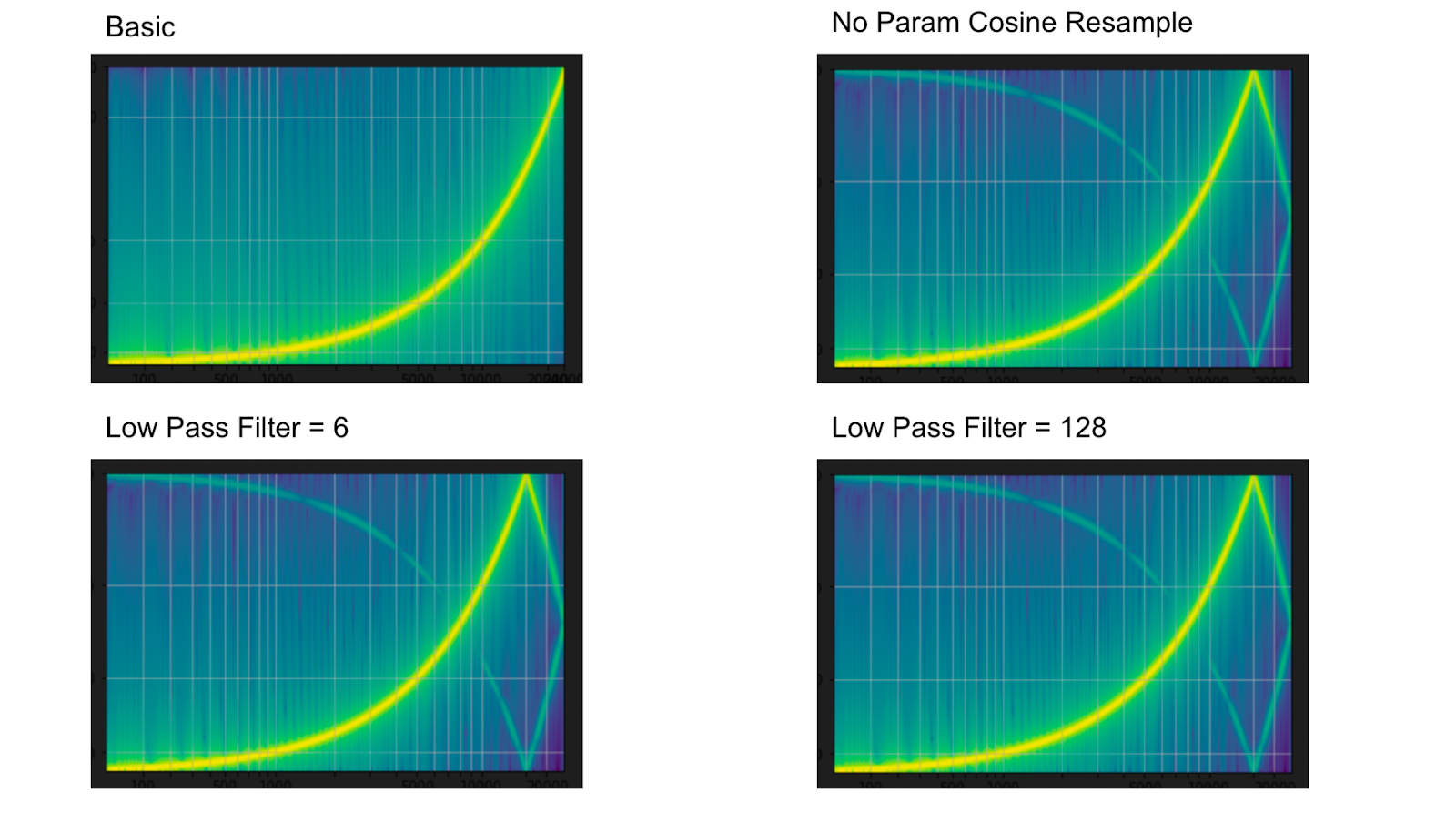 Above: Basic and Low Pass Filter Example Spectrogram from TorchAudio
Filters are not the only thing we can use for resampling. In the example code below, we’ll be using both the default Hann window and the Kaiser window. Both windows serve as ways to automatically filter. Using rolloff for resampling achieves the same goals. In our examples, we’ll take a rolloff of 0.99 and 0.8. A rolloff represents what proportion of the audio will be attenuated.
print("using a window to resample")
hann_window_resampled_waveform = F.resample(waveform, sample_rate, resample_rate, resampling_method="sinc_interpolation")
plot_sweep(resampled_waveform, resample_rate, title="Hann Window Default")
kaiser_window_resampled_waveform = F.resample(waveform, sample_rate, resample_rate, resampling_method="kaiser_window")
plot_sweep(resampled_waveform, resample_rate, title="Kaiser Window Default")
print("user rollof to determine window")
rolloff_resampled_waveform = F.resample(waveform, sample_rate, resample_rate, rolloff=0.99)
plot_sweep(resampled_waveform, resample_rate, title="rolloff=0.99")
rolloff_resampled_waveform = F.resample(waveform, sample_rate, resample_rate, rolloff=0.8)
plot_sweep(resampled_waveform, resample_rate, title="rolloff=0.8")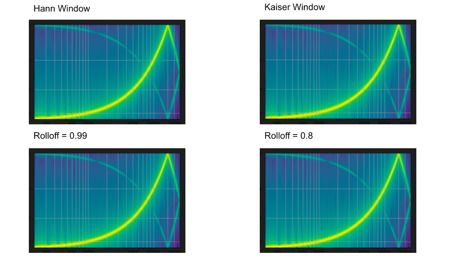 Above: Windowed and Rolloff parameter resampling visualizations from TorchAudio
Audio Feature Extraction with PyTorch TorchAudio
So far we’ve taken a look at how to use torchaudio in many ways to manipulate our audio data. Now let’s take a look at how to do feature extraction with torchaudio. As we have in the two sections above, we’ll start by setting up.
Our setup functions will include functions to fetch the data as well as visualize it like the “effects” section above. We also add some functions for doing Mel scale buckets. We will use Mel scale buckets to make Mel-frequency cepstral coefficients (MFCC), these coefficients represent audio timbre.
import os

import torch
import torchaudio
import torchaudio.functional as F
import torchaudio.transforms as T
import librosa
import matplotlib.pyplot as plt
import requests


_SAMPLE_DIR = "_assets"

SAMPLE_WAV_SPEECH_URL = "https://pytorch-tutorial-assets.s3.amazonaws.com/VOiCES_devkit/source-16k/train/sp0307/Lab41-SRI-VOiCES-src-sp0307-ch127535-sg0042.wav"  # noqa: E501
SAMPLE_WAV_SPEECH_PATH = os.path.join(_SAMPLE_DIR, "speech.wav")

os.makedirs(_SAMPLE_DIR, exist_ok=True)


def _fetch_data():
   uri = [
       (SAMPLE_WAV_SPEECH_URL, SAMPLE_WAV_SPEECH_PATH),
   ]
   for url, path in uri:
       with open(path, "wb") as file_:
           file_.write(requests.get(url).content)


_fetch_data()


def _get_sample(path, resample=None):
   effects = [["remix", "1"]]
   if resample:
       effects.extend(
           [
               ["lowpass", f"{resample // 2}"],
               ["rate", f"{resample}"],
           ]
       )
   return torchaudio.sox_effects.apply_effects_file(path, effects=effects)


def get_speech_sample(*, resample=None):
   return _get_sample(SAMPLE_WAV_SPEECH_PATH, resample=resample)


def plot_spectrogram(spec, title=None, ylabel="freq_bin", aspect="auto", xmax=None):
   fig, axs = plt.subplots(1, 1)
   axs.set_title(title or "Spectrogram (db)")
   axs.set_ylabel(ylabel)
   axs.set_xlabel("frame")
   im = axs.imshow(librosa.power_to_db(spec), origin="lower", aspect=aspect)
   if xmax:
       axs.set_xlim((0, xmax))
   fig.colorbar(im, ax=axs)
   plt.show(block=False)


def plot_waveform(waveform, sample_rate, title="Waveform", xlim=None, ylim=None):
   waveform = waveform.numpy()

   num_channels, num_frames = waveform.shape
   time_axis = torch.arange(0, num_frames) / sample_rate

   figure, axes = plt.subplots(num_channels, 1)
   if num_channels == 1:
       axes = [axes]
   for c in range(num_channels):
       axes[c].plot(time_axis, waveform[c], linewidth=1)
       axes[c].grid(True)
       if num_channels > 1:
           axes[c].set_ylabel(f"Channel {c+1}")
       if xlim:
           axes[c].set_xlim(xlim)
       if ylim:
           axes[c].set_ylim(ylim)
   figure.suptitle(title)
   plt.show(block=False)


def plot_mel_fbank(fbank, title=None):
   fig, axs = plt.subplots(1, 1)
   axs.set_title(title or "Filter bank")
   axs.imshow(fbank, aspect="auto")
   axs.set_ylabel("frequency bin")
   axs.set_xlabel("mel bin")
   plt.show(block=False)
The first thing we’re going to do here is plot the spectrogram and reverse it. The waveform to spectrogram and then back again. Why is converting a waveform to a spectrogram useful for feature extraction? This representation is helpful for extracting spectral features like frequency, timbre, density, rolloff, and more.
We’ll define some constants before we create our spectrogram and reverse it. First, we want to define n_fft, the size of the fast fourier transform, then the window length (the size of the window) and the hop length (the distance between short-time fourier transforms). Then, we’ll call torchaudio to transform our waveform into a spectrogram. To turn a spectrogram back into a waveform, we’ll use the GriffinLim function from torchaudio with the same parameters we used above to turn the waveform into a spectrogram.
# plot spectrogram
waveform, sample_rate = get_speech_sample()
n_fft = 1024
win_length = None
hop_length = 512
# create spectrogram
torch.random.manual_seed(0)
plot_waveform(waveform, sample_rate, title="Original")
spec = T.Spectrogram(
n_fft=n_fft,
win_length=win_length,
hop_length=hop_length,
)(waveform)
plot_spectrogram(spec[0], title="torchaudio spec")
# reverse spectrogram to waveform with griffinlim
griffin_lim = T.GriffinLim(
n_fft=n_fft,
win_length=win_length,
hop_length=hop_length,
)
waveform = griffin_lim(spec)
plot_waveform(waveform, sample_rate, title="Reconstructed")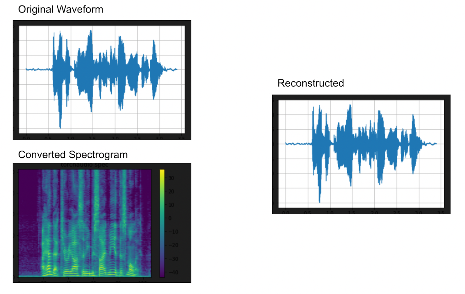 Above: Creating and reversing a spectrogram in PyTorch
Let’s take a look at one of the more interesting things we can do with spectral features, mel-frequency cepstrum. The mel-frequency ceptrsal coefficients (MFCC) represent the timbre of the audio. Before we get started getting these feature coefficients, we’ll define a number of mel filterbanks (256), and a new sample rate to play with.
The first thing we need for MFCC is getting the mel filterbanks. Once we get mel filter banks, we’ll use that to get the mel spectrogram. Now, we’re ready to get the coefficients. First we need to define how many coefficients we want, then we’ll use the mel filterbanks and the mel spectrogram to create an MFCC diagram. This is what our mel spectrogram looks like when reduced to the number of coefficients we specified above.
# mel spectrogram
# mel scale waveforms
# mel scale bins
n_mels = 256
sample_rate = 6000
mel_filters = F.melscale_fbanks(
int(n_fft // 2 + 1),
n_mels=n_mels,
f_min=0.0,
f_max=sample_rate / 2.0,
sample_rate=sample_rate,
norm="slaney",
)
plot_mel_fbank(mel_filters, "Mel Filter Bank - torchaudio")
# mel spectrogram
mel_spectrogram = T.MelSpectrogram(
sample_rate=sample_rate,
n_fft=n_fft,
win_length=win_length,
hop_length=hop_length,
center=True,
pad_mode="reflect",
power=2.0,
norm="slaney",
onesided=True,
n_mels=n_mels,
mel_scale="htk",
)
melspec = mel_spectrogram(waveform)
plot_spectrogram(melspec[0], title="MelSpectrogram - torchaudio", ylabel="mel freq")
n_mfcc = 256
mfcc_transform = T.MFCC(
sample_rate=sample_rate,
n_mfcc=n_mfcc,
melkwargs={
"n_fft": n_fft,
"n_mels": n_mels,
"hop_length": hop_length,
"mel_scale": "htk",
},
)
mfcc = mfcc_transform(waveform)
plot_spectrogram(mfcc[0])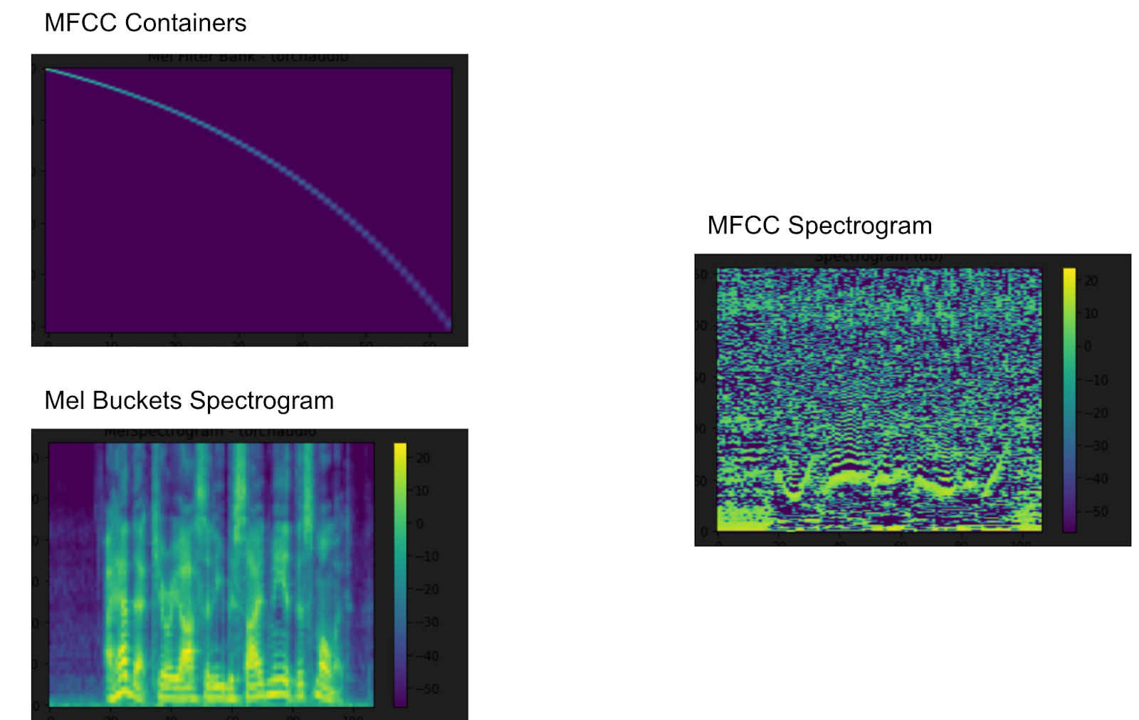 Above: MFCC Feature Extraction of Audio Data with PyTorch TorchAudio
In Summary
In this epic post, we covered the basics of how to use the torchaudio library from PyTorch. We saw that we can use torchaudio to do detailed and sophisticated audio manipulation. The specific examples we went over are adding sound effects, background noise, and room reverb.
TorchAudio also provides other audio manipulation methods as well, such as advanced resampling. In our resampling examples, we showed how to use multiple functions and parameters from TorchAudio’s functional and transform libraries to resample with different filters. We used low-pass filters, roll off filters, and window filters.
Finally, we covered how to use TorchAudio for feature extraction. We showed how to create a spectrogram to get spectral features, reverse that spectrogram with the Griffin-Lim formula, and how to create and use mel-scale bins to get mel-frequency cepstral coefficients (MFCC) features.
If you have any feedback about this post, or anything else around Deepgram, we'd love to hear from you. Please let us know in our GitHub discussions .
More with these tags:
Share your feedback
Was this article useful or interesting to you?
Thank you!
We appreciate your response.

